Plotting maps
Recommended packages:
- tmap: special-purpose package for thematic maps in R. [focus]
- ggplot: most popular package for datavis in R, recent and growing support for maps.
- leaflet: flexible, general purpose package for interactive maps.
- mapview: quick, single-function to interactively view spatial data(frames).
Learn more:
- Stackoverflow.
- Documentation tmap (F1).
- Books: “An Introduction to R for Spatial Analysis and Mapping (2018)”, “Geocomputation with R (full-text)”, “Data Visualization. A practical introduction” (full text).
- Datacamp courses.
library(BelgiumMaps.StatBel)
library(mapview)
library(sf)
library(tmap)
library(readr)
library(dplyr)
library(ggplot2)Thematic maps with tmap
In an nutshell:
- Quick thematic map:
qtm() - Build map in layers with lots of control and options:
tm_shape(),tm_fill(),tm_borders(), etc. - Cherry-on-top: switch between interactive and static plotting with
tmap_mode('view')andtmap_mode('plot').
Some resources:
- Getting started with tmap
- https://geocompr.robinlovelace.net/adv-map.html
- Background and walkthrough: Tennekes, M., 2018, tmap: Thematic Maps in R, Journal of Statistical Software, 84(6), 1-39.
Already showed some examples, here extra focus on:
- “Layered” building of maps.
- Binning and color scales
- Multiple (styled) borders
- Multiple maps
Tip: for final tweaks, save map as SVG in Inkscape.
# load boundary for entire BE
data("BE_ADMIN_BELGIUM")
be <- st_as_sf(BE_ADMIN_BELGIUM)
# load municipal boundaries
data("BE_ADMIN_MUNTY")
munip_map <- st_as_sf(BE_ADMIN_MUNTY)
# load fiscal income data on municipal level
munip_data <- read_csv(
file = 'data/fiscal_incomes_2016.csv',
col_types = cols(
munip_label = col_character(),
munip_nis = col_character(),
n_inhabitants = col_integer(),
income_mean = col_integer() ))
# add map and income data together on muncipal level
munip <- left_join(
munip_map, munip_data,
by = c('CD_MUNTY_REFNIS' = 'munip_nis'))Building maps in layers
tm_shape(munip) +
tm_borders()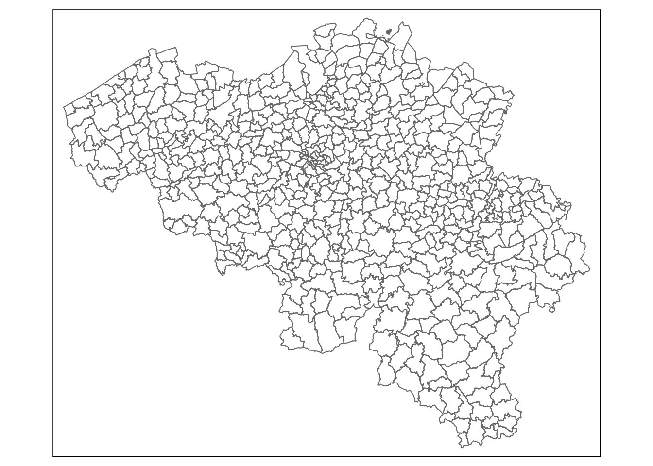
tm_shape(munip) +
tm_fill(col = 'income_mean', title = 'Mean income (2016)')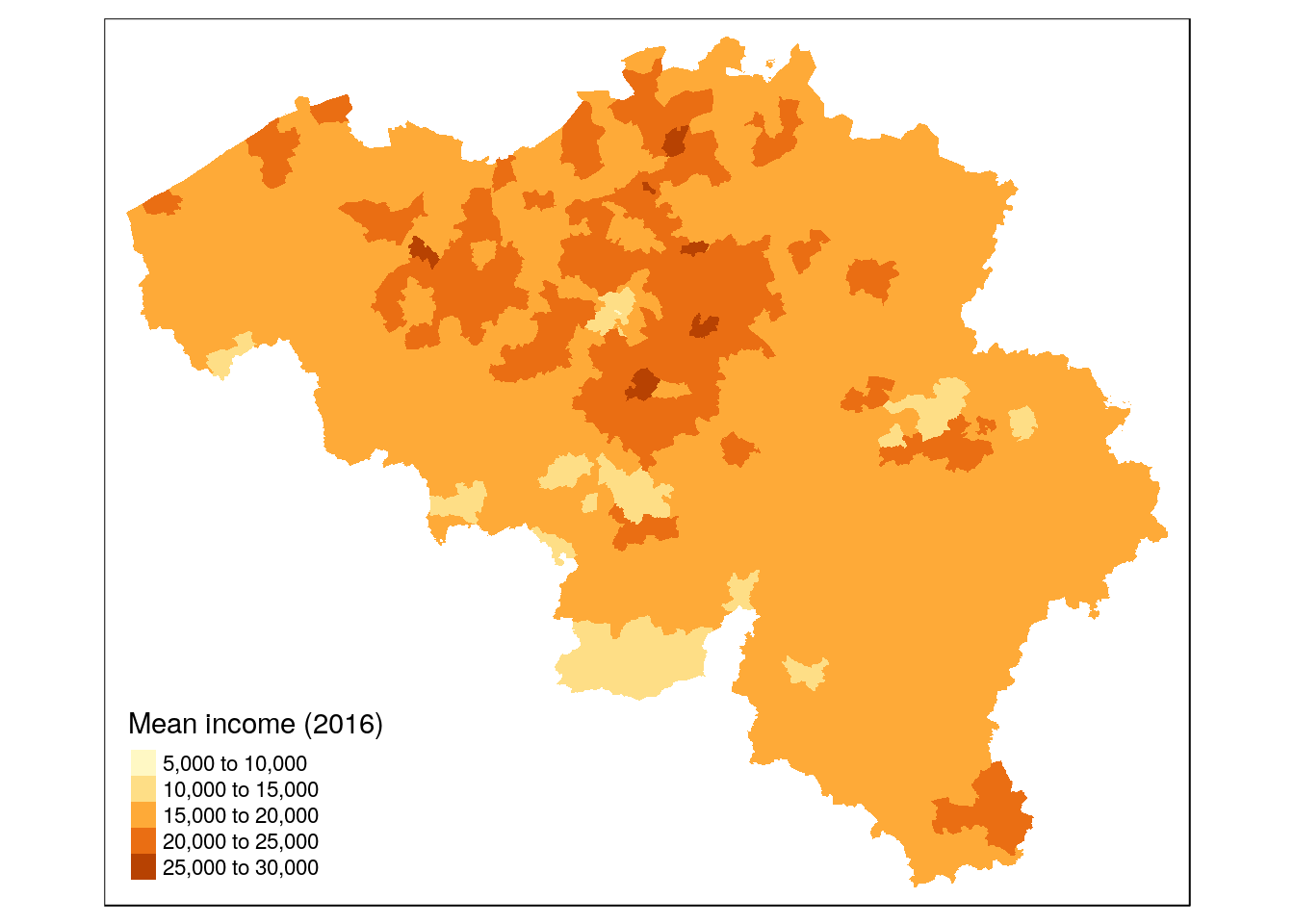
tm_shape(munip) +
tm_borders() +
tm_fill(col = 'income_mean', title = 'Mean income (2016)')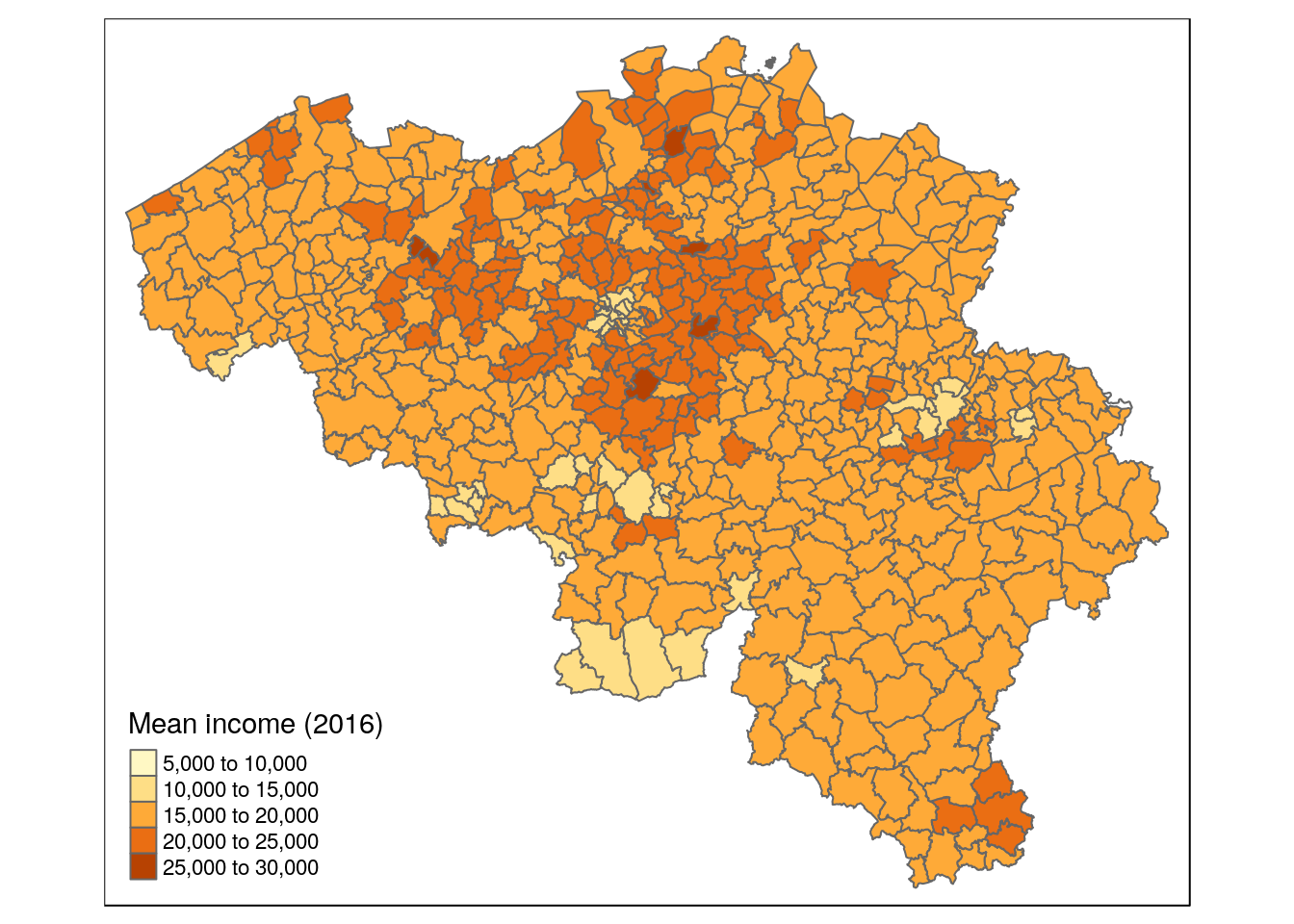
tm_shape(munip) +
tm_borders(col = 'white', lwd = 0.3) +
tm_fill(col = 'income_mean', title = 'Mean income (2016)')
tm_shape(munip) +
tm_borders(col = 'white', lwd = 0.3) +
tm_fill(col = 'income_mean', title = 'Mean income (2016)', legend.hist = TRUE) +
tm_legend(legend.outside = TRUE)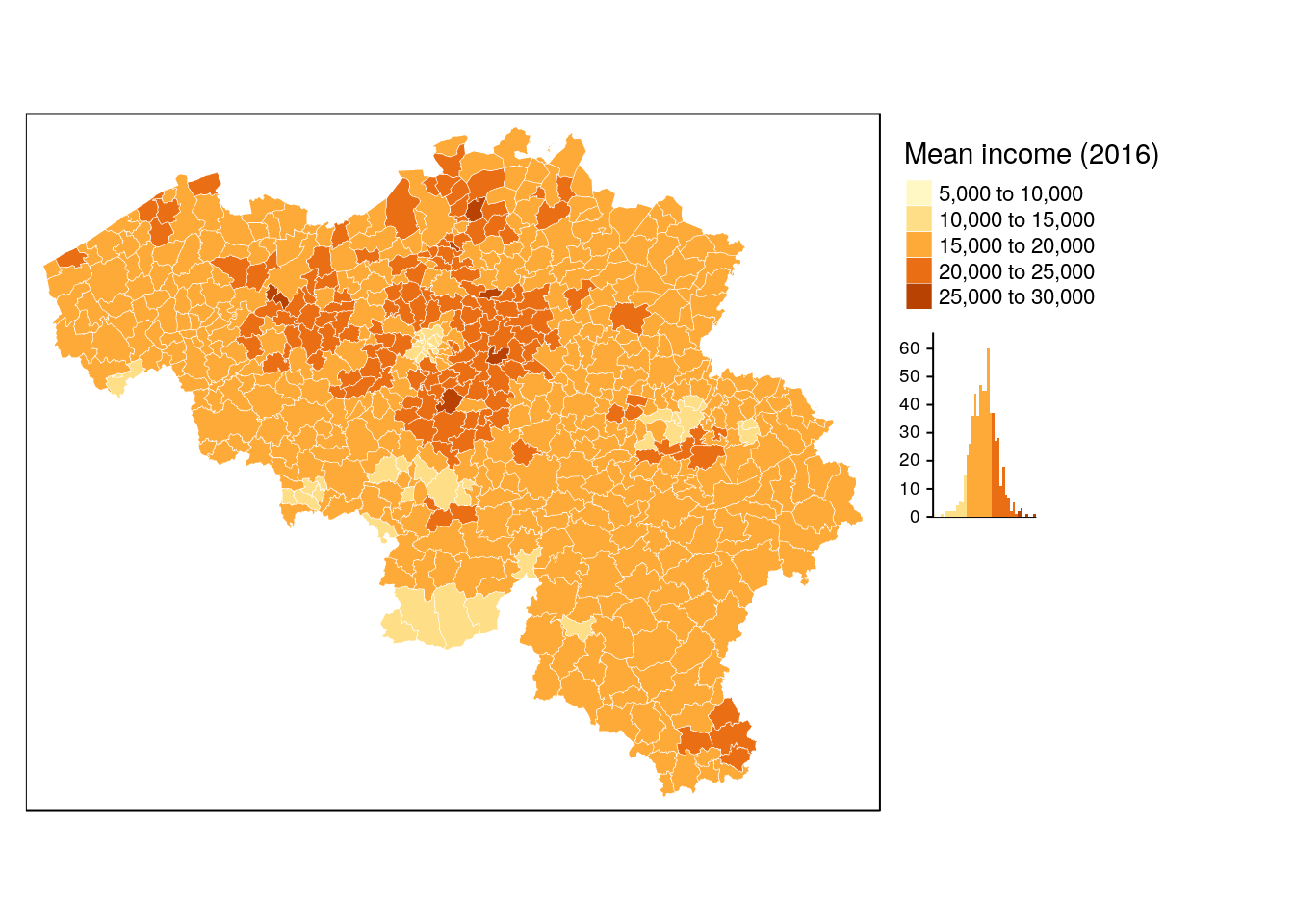
tm_shape(munip) +
tm_borders(col = 'white', lwd = 0.3) +
tm_fill(col = 'income_mean', title = 'Mean income (2016)', legend.hist = TRUE) +
tm_legend(legend.outside = TRUE) +
tm_layout(frame = FALSE) +
tm_credits('Source: Statbel, Fiscale statistiek van de inkomsten 2005-2016', position = 'left')
tm_shape(munip) +
tm_borders(col = 'white', lwd = 0.3) +
tm_fill(col = 'income_mean', title = 'Mean income (2016)', legend.hist = FALSE) +
tm_legend(legend.outside = FALSE) +
tm_layout(frame = FALSE) +
tm_credits('Source: Statbel, Fiscale statistiek van de\ninkomsten 2005-2016', position = 'center') +
tm_style_grey(legend.format = list(text.separator= "-")) +
tm_logo("data/hiva_logo_400x400.png")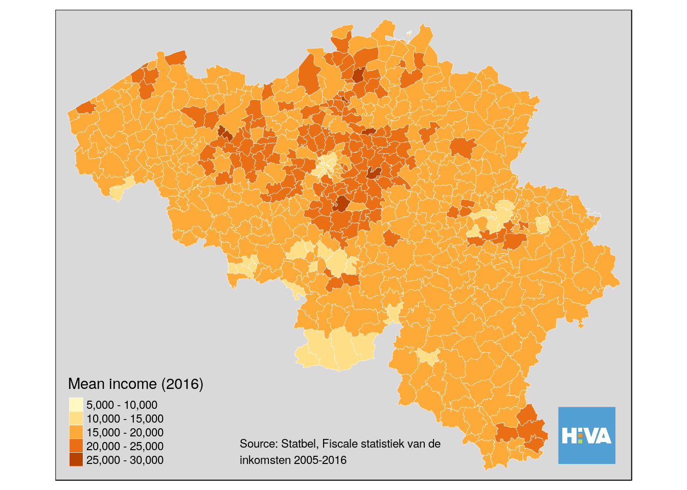
Add layers using objects
be_income <- tm_shape(munip) +
tm_borders(col = 'white', lwd = 0.3) +
tm_fill(col = 'income_mean', title = 'Mean income (2016)', legend.hist = FALSE) +
tm_legend(legend.outside = FALSE)
be_income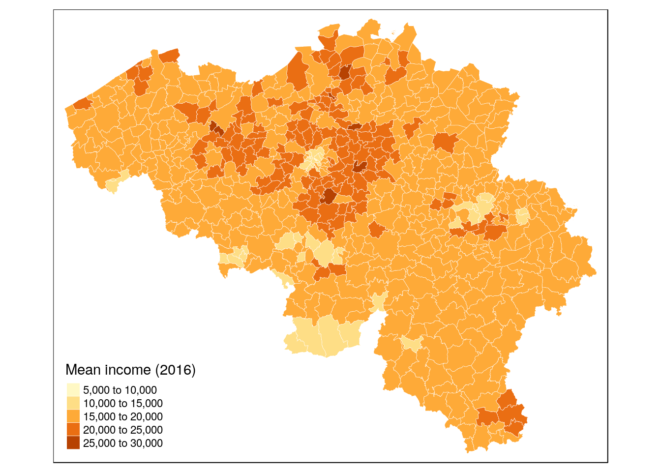
be_income_style <- be_income +
tm_layout(frame = FALSE) +
tm_credits('Source: Statbel, Fiscale statistiek van de\ninkomsten 2005-2016', position = 'center') +
tm_style_grey(legend.format = list(text.separator= "-")) +
tm_logo("data/hiva_logo_400x400.png", height = 2) + # scale down logo size a bit
tm_layout(scale = 0.8) # reduce over text-size## Warning in tm_style_grey(legend.format = list(text.separator =
## "-")): tm_style_grey is deprecated as of tmap version 2.0. Please use
## tm_style("grey", ...) insteadbe_income_style## Note that tm_style("grey") resets all options set with tm_layout, tm_view, tm_format, or tm_legend. It is therefore recommended to place the tm_style element prior to the other tm_layout/tm_view/tm_format/tm_legend elements.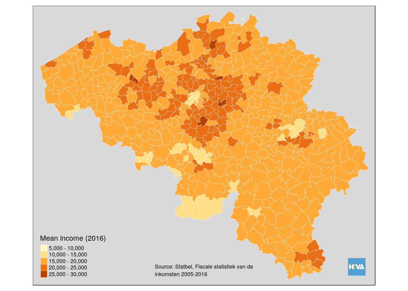
save_tmap(be_income_style, 'output/be_income_muni_2016.png', width = 1920, height = 1080)## Warning in save_tmap(be_income_style, "output/be_income_muni_2016.png", :
## save_tmap is deprecated as of tmap version 2.0. Please use tmap_save
## instead## Note that tm_style("grey") resets all options set with tm_layout, tm_view, tm_format, or tm_legend. It is therefore recommended to place the tm_style element prior to the other tm_layout/tm_view/tm_format/tm_legend elements.## Map saved to /home/rstudio/projects/thematic-maps-r/output/be_income_muni_2016.png## Resolution: 1920 by 1080 pixels## Size: 6.4 by 3.6 inches (300 dpi)Styled (multiple) borders
data("BE_ADMIN_PROVINCE")
prov <- st_as_sf(BE_ADMIN_PROVINCE)be_income_prov <- be_income +
tm_shape(prov) +
tm_borders(col = 'black', lwd = .2)
be_income_prov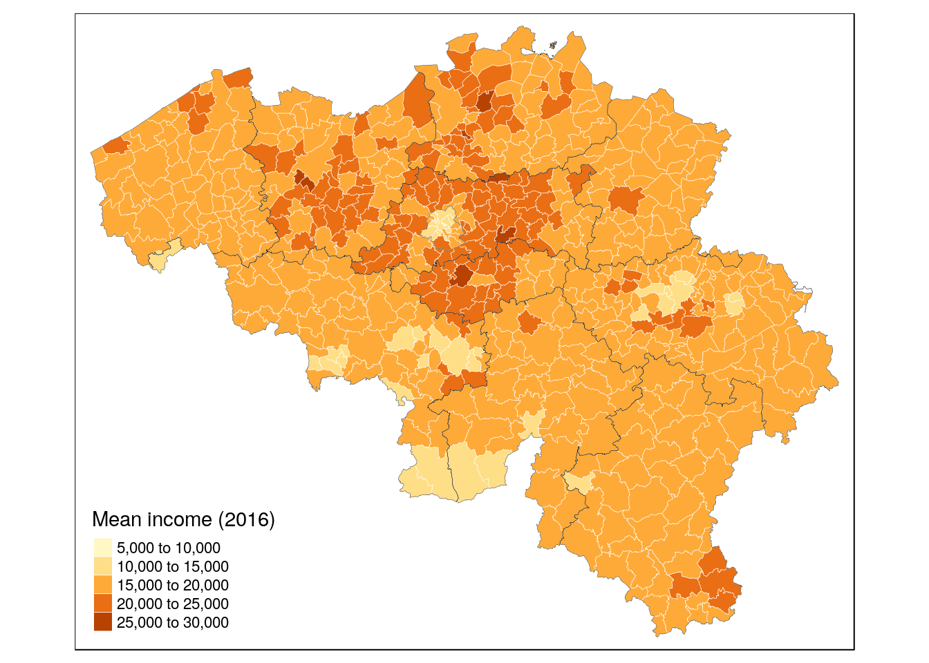
Binning and color palettes
- Choice of binning intervals matters.
- Choise of color palette matters, cf. colorbrewer: sequential, diverging, and qualitative color palettes.
min(munip$income_mean)## [1] 8835max(munip$income_mean)## [1] 28348tm_shape(munip) +
tm_fill(col = 'income_mean',
title = 'Mean income (2016)',
breaks = c(0, 20000, 25000, 30000)) +
tm_borders(col = 'white', lwd = .5)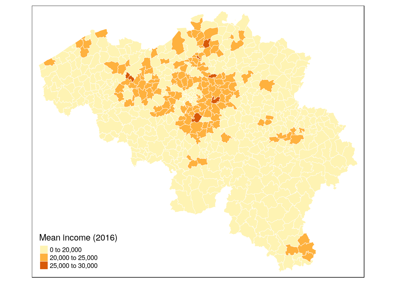
tm_shape(munip) +
tm_fill(col = 'income_mean',
title = 'Mean income (2016)',
n=20, # detailed breaks!
legend.hist = TRUE) +
tm_borders(col = 'white', lwd = .5) +
tm_legend(legend.outside = TRUE, legend.outside.position="right")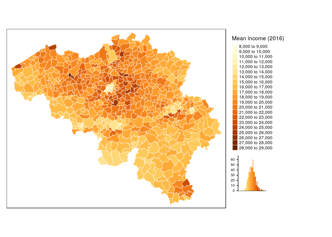
be_income_div <- tm_shape(munip) +
tm_fill(col = 'income_mean',
title = 'Mean income (2016)',
n = 20,
palette = "RdBu", auto.palette.mapping = FALSE, # diverging pallette!
legend.hist = TRUE) +
tm_borders(col = 'white', lwd = .5) +
tm_legend(legend.outside = TRUE, legend.outside.position="right") +
tm_shape(be) +
tm_borders(col = 'black', lwd = 0.3) +
tm_layout(frame = FALSE)## Warning: The argument auto.palette.mapping is deprecated. Please use
## midpoint for numeric data and stretch.palette for categorical data to
## control the palette mapping.be_income_div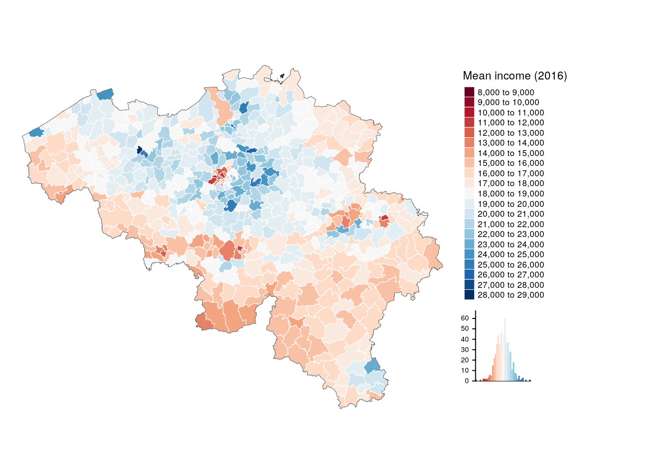
Multiple maps / facets
Facets: more info in getting started document online.
tm_shape(munip) +
tm_borders(col = 'white', lwd = .5) +
tm_fill(col = c("income_mean", 'n_inhabitants')) +
tm_layout(legend.position = c('left', 'bottom'))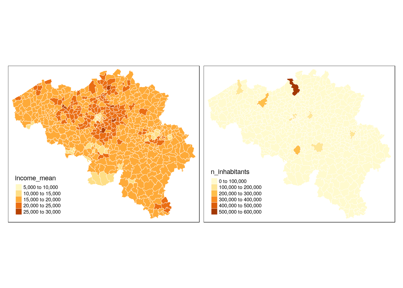
m_be_income <- tm_shape(munip) +
tm_borders(col = 'white', lwd = .5) +
tm_fill(col = "income_mean", title = 'Mean income (2016)')
m_be_pop <- tm_shape(munip) +
tm_borders(col = 'white', lwd = .5) +
tm_fill(col = "n_inhabitants", title = "Population (2010)")
tmap_arrange(m_be_income, m_be_pop)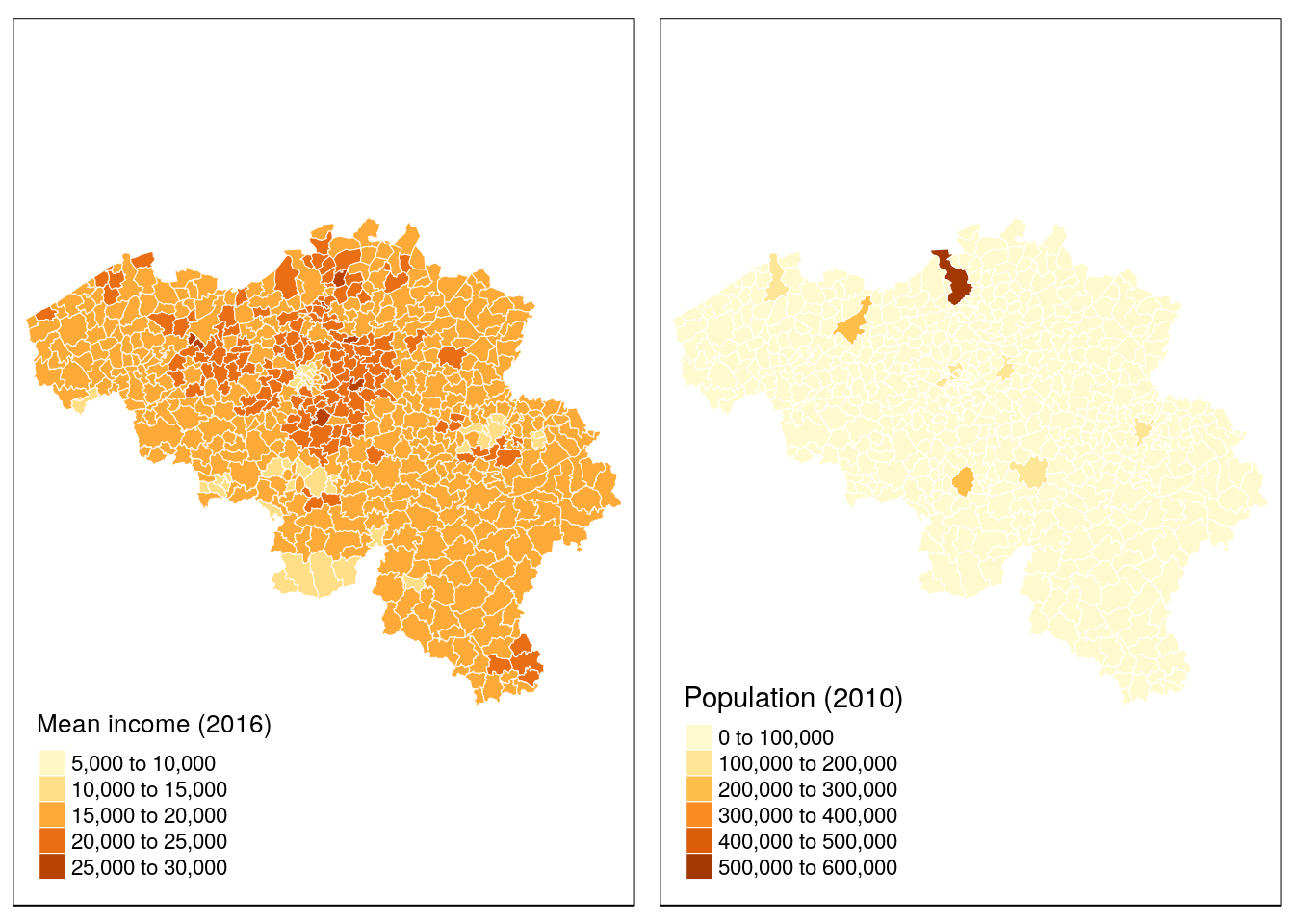
tmap interactive mode
tmap_mode('view')
be_income_div