What we will be working towards
Illustrating through exampes common steps for common thematic maps:
- Get an appropriate blank map.
- Load and add “regular” data.
- Manipulate (spatial) data.
- Plot map.
Socio-economic clusters
# [1] Get blank map (of Belgian muncipalities)
data("BE_ADMIN_MUNTY")
munip_map <- st_as_sf(BE_ADMIN_MUNTY)

# [2] Load and add data-of-interest (Excel-file of socio-economic cluster-type of muncipality)
munip_data <- read_excel('data/muni_typology.xlsx', col_types = 'text')
munip <- left_join(munip_map, munip_data, by = c('CD_MUNTY_REFNIS' = 'gemeente_nis_code'))

# [3] Manipulate data (not needed)

# [4] Plot map
qtm(munip, fill = 'hoofdcluster_lbl', fill.title = 'Socio-economic cluster')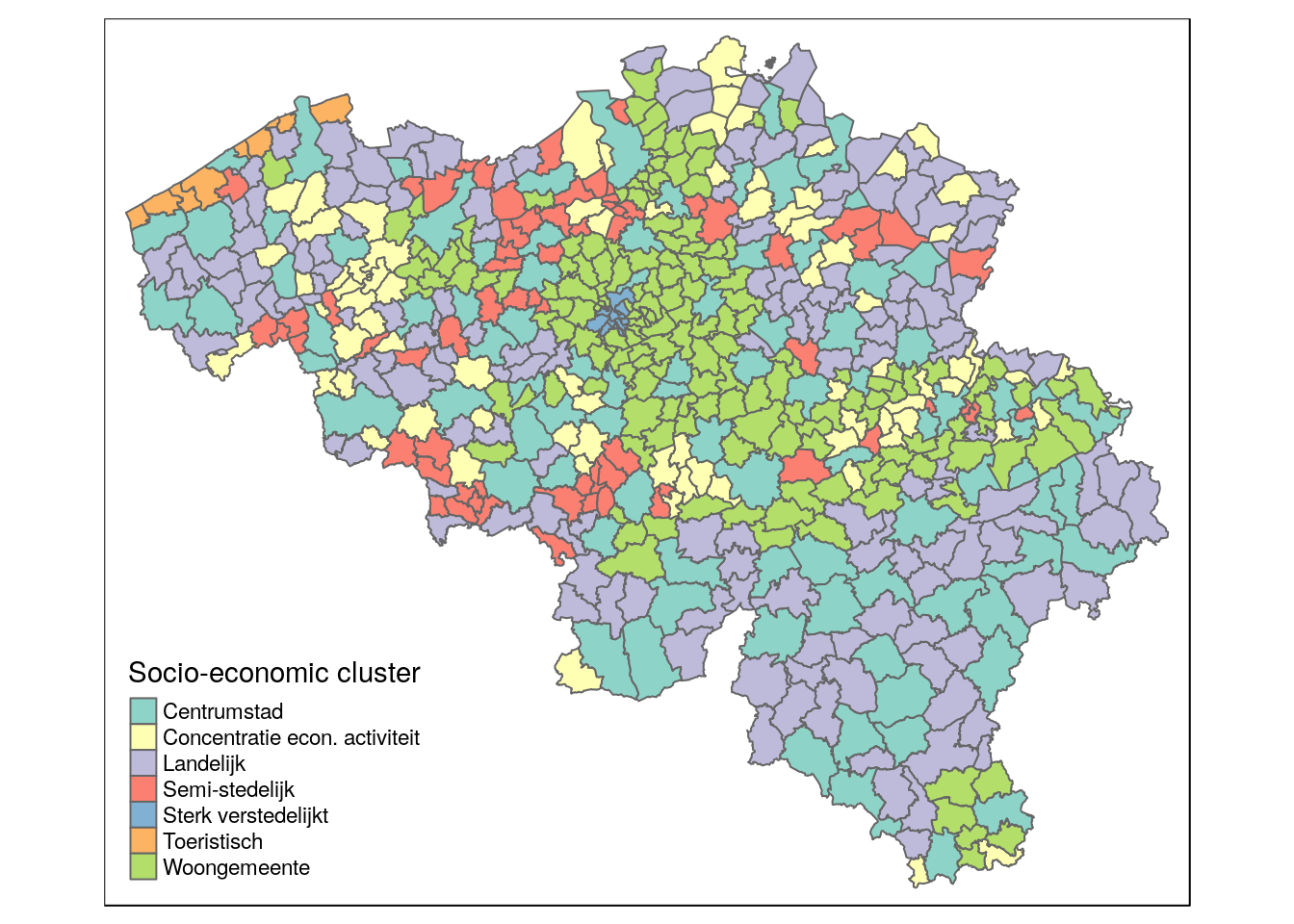
Part-time work in the EU
# [1] Get blank map (of EU countries directly from Eurostat)
map_data <- get_eurostat_geospatial(resolution = "60", nuts_level = "0")
map_data <- st_crop(map_data, c(xmin=-10, xmax=45, ymin=36, ymax=71))

# [2] Load and add data-of-interest (Excel-file with % part-time workers, from Eurostat)
worktime_data <- read_excel('data/eurostat_workingtime_2017.xlsx')
worktime <- left_join(map_data, worktime_data, by = c('CNTR_CODE' = 'geo'))

# [3] Manipulate data (not needed)

# [4] Plot map
qtm(worktime, fill = 'values', fill.title = 'Percentage part-time')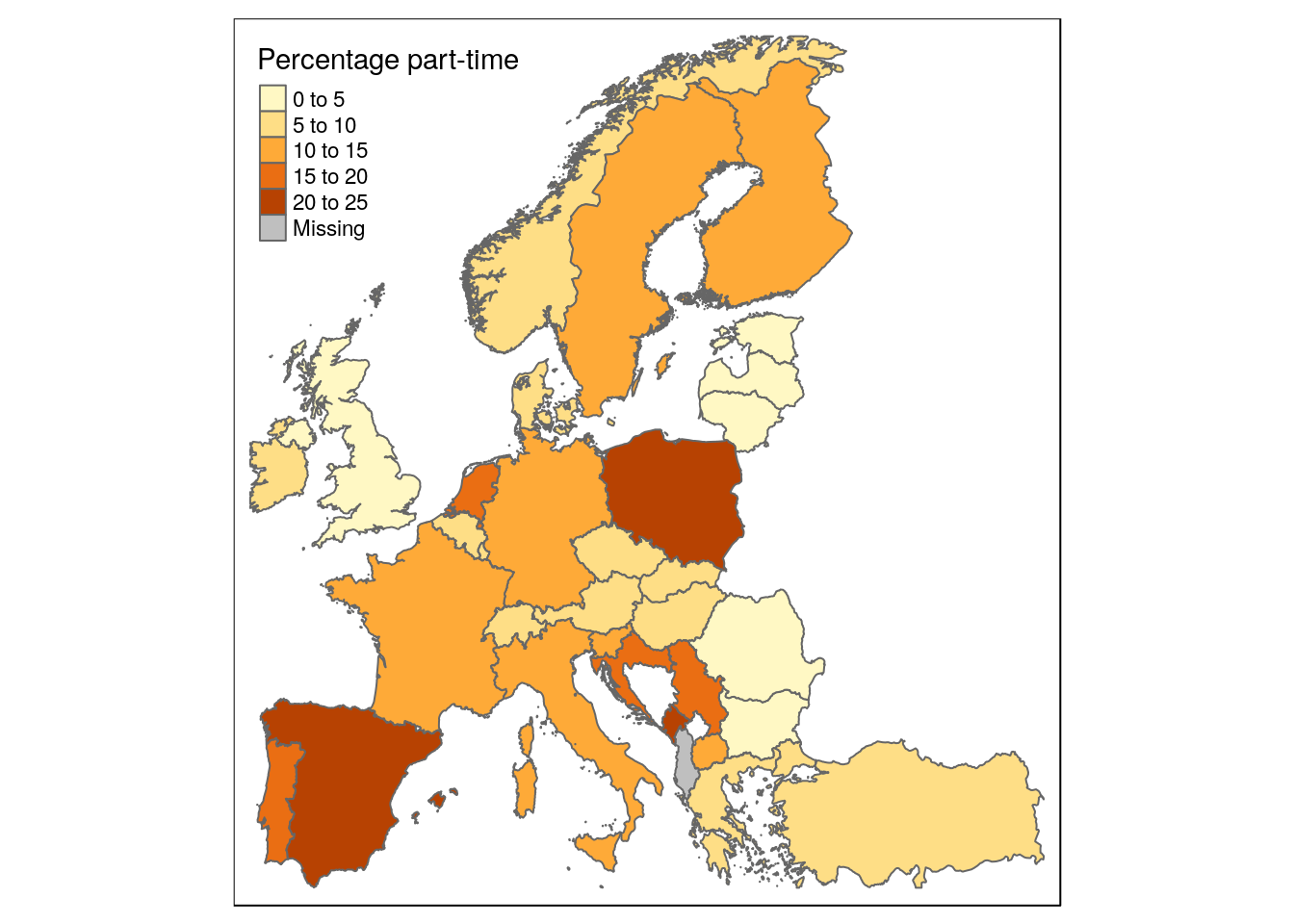
Mean income in Limburg (PPP)
# [1] Get blank map (of Belgian muncipalities)
data("BE_ADMIN_MUNTY")
munip_map <- st_as_sf(BE_ADMIN_MUNTY)

# [2] Load and add data-of-interest (Stata file with fiscal income data on municipal level).
munip_data <- read_dta('data/fiscal_incomes_2016.dta')
munip <- left_join(munip_map, munip_data, by = c('CD_MUNTY_REFNIS' = 'munip_nis'))

# [3] Manipulate (spatial) data (select muncipalities in Limburg, and convert to PPP).
limburg <- munip %>%
  filter(TX_PROV_DESCR_NL == 'Provincie Limburg') %>%
  mutate(income_mean_ppp = income_mean * 0.794)

# [4] Plot map.
qtm(limburg, fill = 'income_mean_ppp', fill.title = 'Mean income (2016, PPP)')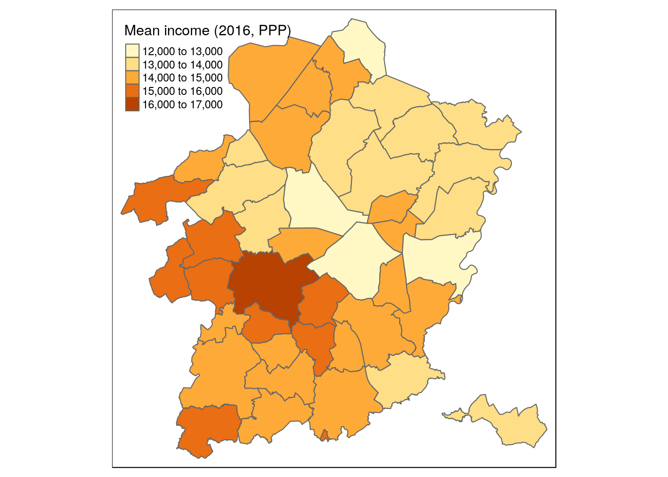
Interactive map of income in Brussels
# [1] Get blank map (of Belgian muncipalities)
data("BE_ADMIN_MUNTY")
munip_map <- st_as_sf(BE_ADMIN_MUNTY)

# [2] Load and add data-of-interest (Stata file with fiscal income data on municipal level).
munip_data <- read_dta('data/fiscal_incomes_2016.dta')
munip <- left_join(munip_map, munip_data, by = c('CD_MUNTY_REFNIS' = 'munip_nis'))

# [3] Manipulate (spatial) data (select muncipalities in Limburg, and convert to PPP).
income_vl <- munip %>% filter(TX_RGN_DESCR_NL == 'Brussels Hoofdstedelijk Gewest')

# [4] Plot (interactive) map.
bins <- c(0, 5000, 10000, 15000, 20000, 25000, 30000) # intervals scale & color range
color_range <- colorBin("YlOrRd", domain = income_vl$income_mean, bins = bins)

leaflet(income_vl) %>%
  addProviderTiles(providers$CartoDB.Positron) %>%
  addPolygons(fillColor = ~color_range(income_mean), color = "black", weight = 1, opacity = 1) %>%
  addLegend(values = ~income_mean, title = 'Mean income (2016)', pal = color_range)