Manipulating (spatial) data
Two types of data-manipulation:
- spatial data-manipulations: spatial cropping, union, aggregation, etc.
- ‘regular’ data-manipulations: combine categories, calculate percentage of population, etc.
… but same syntax and in one dataframe.
PS: always an option, do (2) in SAS, Stata, etc. before reading and joining data (previous step).
library(rgdal)      # provides readOGR() to read in spatial data
library(BelgiumMaps.StatBel)
library(sf)
library(tmap)       # plot thematic map with qtm()
library(dplyr)      # general data-manipulation
library(stringr)    # string-operations str_sub()
library(readr)      # read CSV-file read_csv()
Ex. Select specific provinces
data("BE_ADMIN_MUNTY")
map_muni <- st_as_sf(BE_ADMIN_MUNTY)
data_muni <- read_csv('data/muni_typology.csv', col_types = cols(.default = col_character()))
muni <- left_join(map_muni, data_muni, by = c('CD_MUNTY_REFNIS' = 'gemeente_nis_code'))
antw_luik <- muni %>%
filter(TX_PROV_DESCR_NL %in% c('Provincie Antwerpen', 'Provincie Luik'))
qtm(antw_luik, fill = 'hoofdcluster_lbl', fill.title = 'Socio-economic cluster')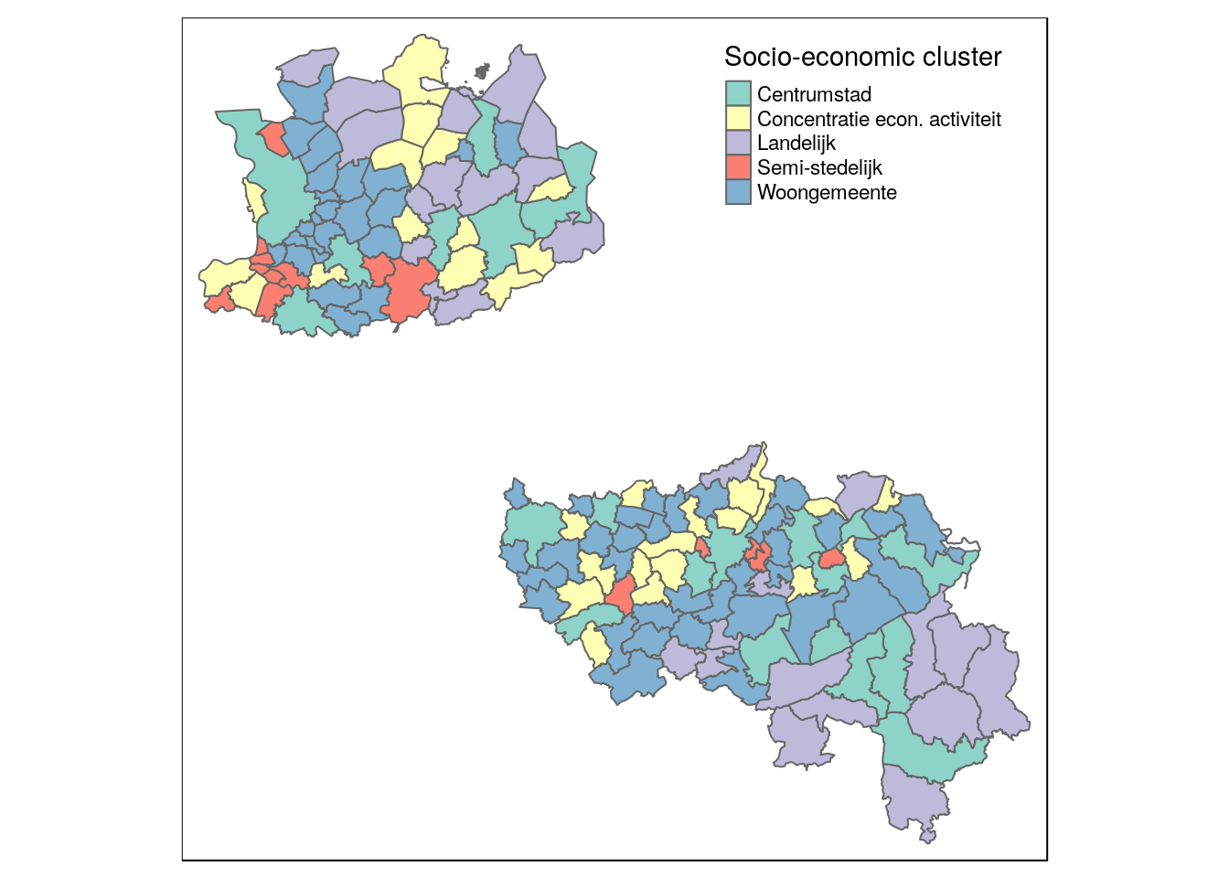
Ex. Spatial aggregation
qtm(muni, fill = 'hoofdcluster_lbl', fill.title = 'Socio-economic cluster')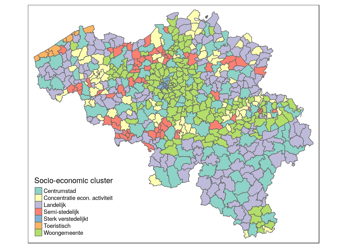
# group all muncipalities together in contiuous spatial area's, if they share the same cluster
muni_clusterd <- muni %>%
  group_by(hoofdcluster_lbl) %>%
  tally()
qtm(muni_clusterd, fill = 'hoofdcluster_lbl', fill.title = 'Socio-economic cluster')
Ex. Covert muncipal income in PPP
# load municipal boundaries
data("BE_ADMIN_MUNTY")
munip_map <- st_as_sf(BE_ADMIN_MUNTY)

# load fiscal income data on municipal level
munip_data <- read_csv(
  file = 'data/fiscal_incomes_2016.csv',
  col_types = cols(
    munip_label = col_character(),
    munip_nis = col_character(),
    n_inhabitants = col_integer(),
    income_mean = col_integer() ))

# add map and income data together on muncipal level
munip <- left_join(
  munip_map, munip_data,
  by = c('CD_MUNTY_REFNIS' = 'munip_nis'))
qtm(munip, fill = 'income_mean', fill.title = 'Mean income (2016)')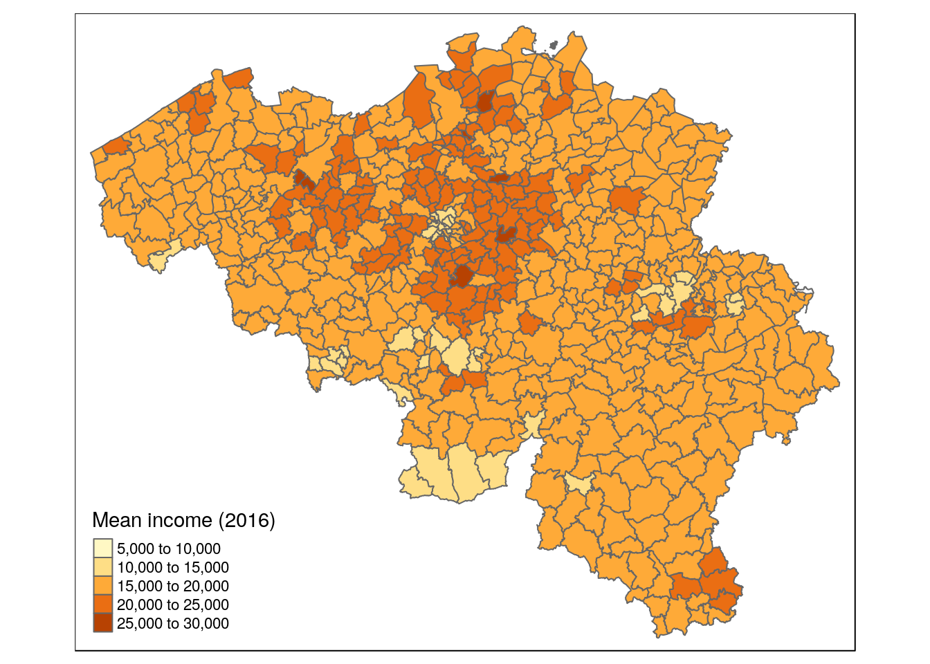
# Convert to Purchasing Power Parity (new variable "income_mean_ppp")
# 2016 Euro-PPP for BE https://data.oecd.org/conversion/purchasing-power-parities-ppp.htm

munip <- munip %>%
  mutate(income_mean_ppp = income_mean * 0.794)
qtm(munip, fill = 'income_mean_ppp', fill.title = 'Mean income (2016, PPP)')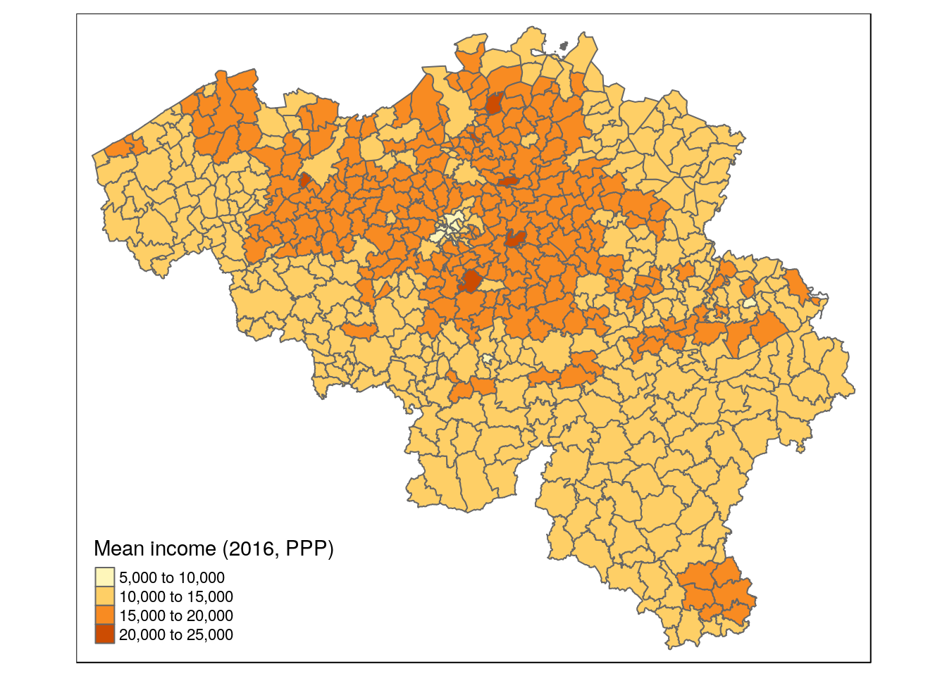
Ex. Calculate, filter and plot on quantiles
# base R function to calculate quantiles (here quartile)
income_quartiles <- quantile(munip$income_mean)
income_quartiles
## 0% 25% 50% 75% 100%
## 8835 16825 18454 20032 28348# make new variable, classifying muncicipalities by mean income quartile ("income_quartile")
munip <- munip %>%
mutate(income_quartile = cut(income_mean, income_quartiles, labels = c('0-25%', '26-50%', '51-75%', '76-100%')))qtm(munip, fill = 'income_quartile', fill.palette = '-Reds',
fill.title = 'Mean income quartiles (2016)')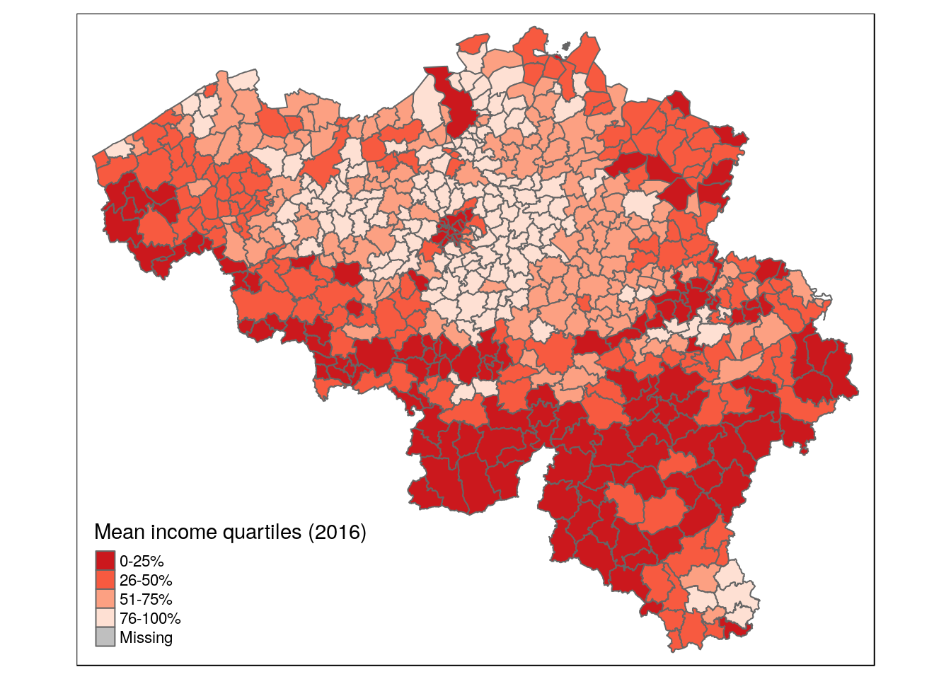
# Select only the muncipalities in the bottom quartile (0-25%)
munip_min25 <- munip %>%
  filter(income_quartile == '0-25%')

qtm(munip_min25, fill = 'income_mean', fill.palette = '-Reds',
    fill.title = 'Mean municipal income in\nbottom quartile (2016)')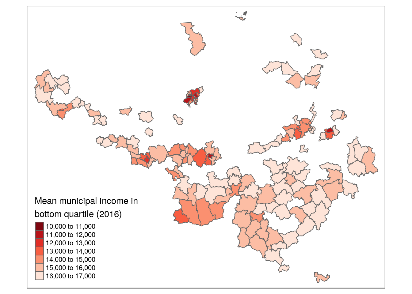
Ex. Aggregate municipal income to district-level
# aggregate spatially _and_ data-wise (take mean of income)
munip_district <- munip %>%
  group_by(TX_ADM_DSTR_DESCR_NL) %>%
  summarise(
    income_mean_aggr = mean(income_mean),
    income_mean_ppp_aggr = mean(income_mean_ppp))
qtm(munip_district, fill = 'income_mean_ppp_aggr', fill.title = 'Mean income (2016, PPP)')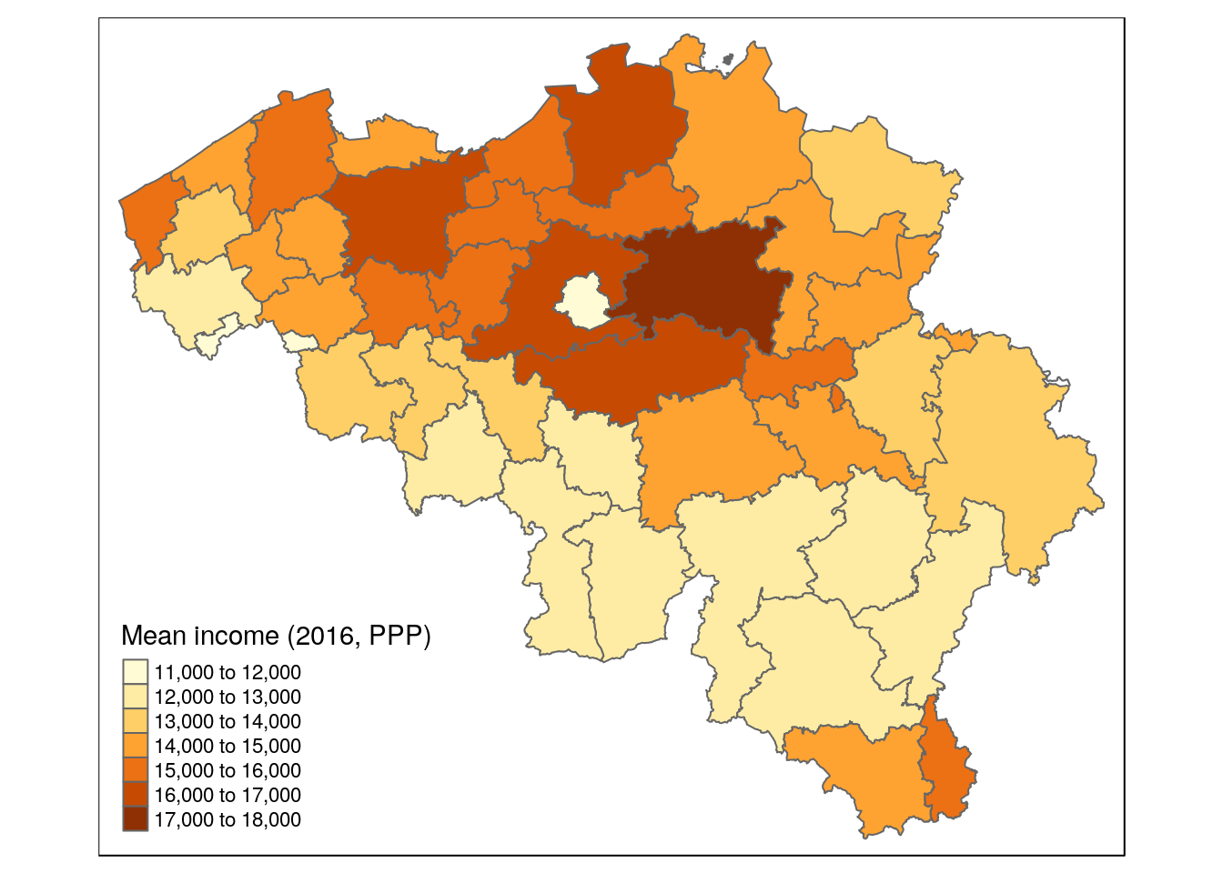
Ex. Immovable Heritage plans
# load spatial boundaries with readOGR()
heritage <- readOGR('data/heritage_plans', layer = 'heritage_plans')
## OGR data source with driver: ESRI Shapefile
## Source: "/home/rstudio/projects/thematic-maps-r/data/heritage_plans", layer: "heritage_plans"
## with 713 features
## It has 6 fields
## Integer64 fields read as strings: IDheritage <- st_as_sf(heritage)# Manipulate: get the start year of the heritage mgmt plan
# using dplyr and str_sub() from stringr
heritage <- heritage %>%
# get year substring (1st to 4th character) and create variable "start_year"
mutate(start_year = str_sub(STARTDATUM, start = 1, end = 4)) # quick thematic map, with color based on start-year, in sequential gradient of blues
heritage_year <- qtm(heritage, fill = 'start_year', fill.palette = 'Blues')
heritage_year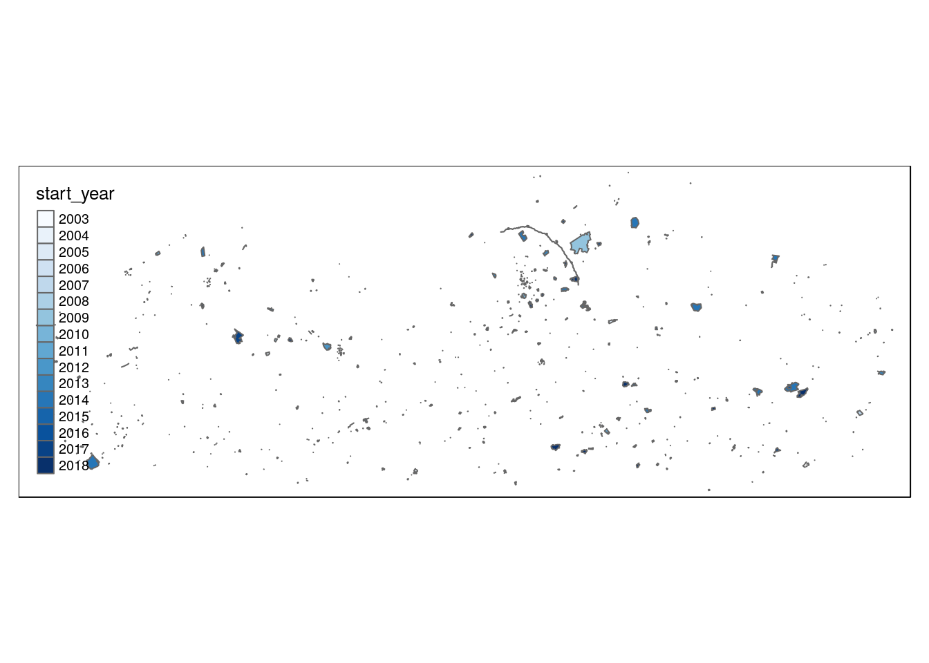
# plot thematic map again, but in tmap interactive mode
tmap_mode('view')
heritage_year
tmap_mode('plot')