Getting your blank maps
We need to have “bank maps” to color in. Two sources:
- Dowloaded file.
- Provided through an R-package [focus].
Points of attention:
- We want sf-objects. Frequently already right format, or convert using
st_as_sf(). - Reduce large map to what you need: filter, crop, or limit.
- Pay attention to included identifier.
# load general packages used below
library(ggplot2)
library(sf)
library(tmap)
library(mapview)
Get maps from downloaded file
Formats: Shapefiles, GeoJSON, KML, etc.
Recommended:
- Use
readOGR()in the rgdal-package: hard to find a format not covered. - Convert to simple features-object using
Semi-random example: download the open-data spatial boundaries of the management plans of the Flemish organization for Immovable Heritage.
library(rgdal)
heritage <- readOGR('data/heritage_plans', layer = 'heritage_plans')
## OGR data source with driver: ESRI Shapefile
## Source: "/home/rstudio/projects/thematic-maps-r/data/heritage_plans", layer: "heritage_plans"
## with 713 features
## It has 6 fields
## Integer64 fields read as strings: IDheritage <- st_as_sf(heritage)qtm(heritage)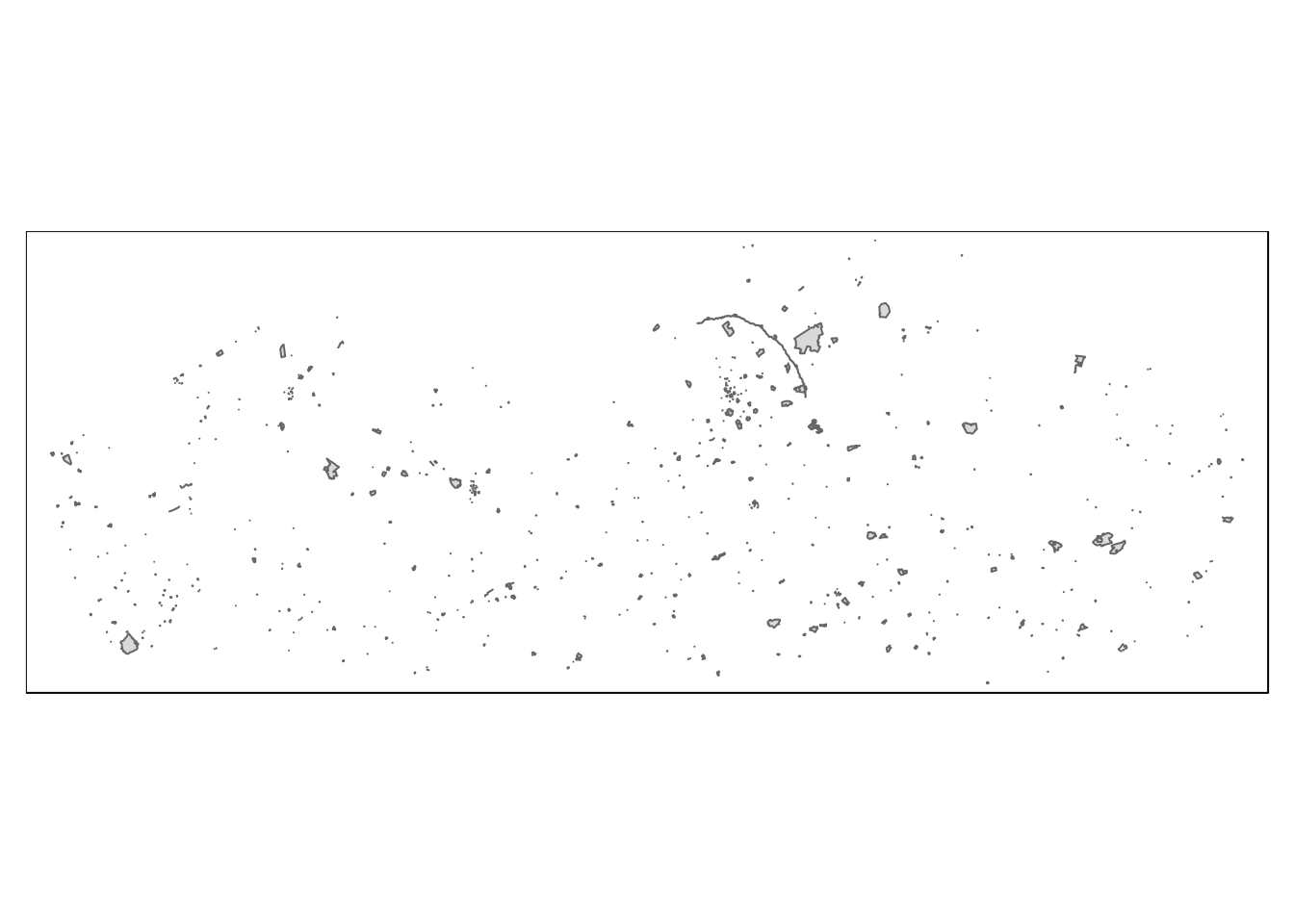
mapview(heritage)Get maps through R-packages
Belgium
BelgiumMaps.StatBel by Jan Wijfels (bnosac): convenient R package bundeling spatial open data on Belgian administrative boundaries.
Load package (library(BelgiumMaps.StatBel)) and then use data() to load the spatial data for the administrative level you need:
- BE_ADMIN_SECTORS: statistical sector / statistische sector
- BE_ADMIN_MUNTY: municipality / gemeente
- BE_ADMIN_DISTRICT: district / arrondissement
- BE_ADMIN_PROVINCE: province / provincie
- BE_ADMIN_REGION: region / regio
- BE_ADMIN_BELGIUM: country / land
Important: the data always contains a variable/column with the NIS-code, named “CD_[level]_REFNIS“. E.g. CD_PROV_REFNIS, CD_RGN_REFNIS, CD_MUNTY_REFNIS. With NIS-codes in your data, you can merge on each level. It also contains NUTS-codes (not demonstrated).
library(BelgiumMaps.StatBel)
data("BE_ADMIN_PROVINCE") # load spatial object for provincial level
provinces <- st_as_sf(BE_ADMIN_PROVINCE) # convert to sf-object
qtm(provinces) # plot with tmap
data("BE_ADMIN_MUNTY")
munip <- st_as_sf(BE_ADMIN_MUNTY)
qtm(munip)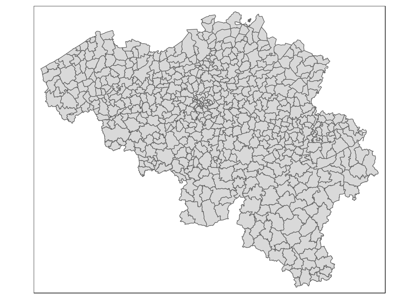
Europe
The eurostat package allows you to directly download, analyse and visualise data from Eurostat in R, including their blank maps of EU-member countries:
- Use the function
get_eurostat_geospatial()to download. - Choose the NUTS level: “0” (countries), “1” (regions, i.e. Flanders), “2” (sub-region, BE: provinces), “3” (sub-sub-region, BE: arrondissment).
- Choose the level of detail: “60” (1:60million), “20” (1:20million), “10” (1:10million), “01” (1:1million). More detail for more zoomed-in maps (longer download, but cached).
- Identifier: NUTS (“NUTS_ID”).
- sf-object by default, no
st_as_sf()needed. - Warning: not EU-member (+ NO, TR, etc.), not on the map!
library(eurostat)
eu_nuts0 <- get_eurostat_geospatial(
  resolution = "60", # detail
  nuts_level = "0") # NUTS 0-3

eu_nuts2 <- get_eurostat_geospatial(
  resolution = "60", # detail
  nuts_level = "2") # NUTS 0-3
qtm(eu_nuts0)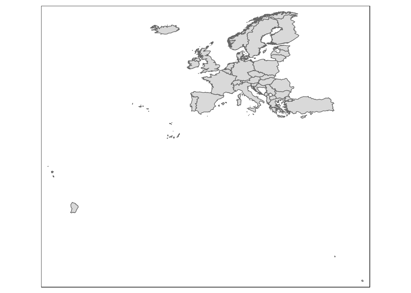
qtm(eu_nuts2)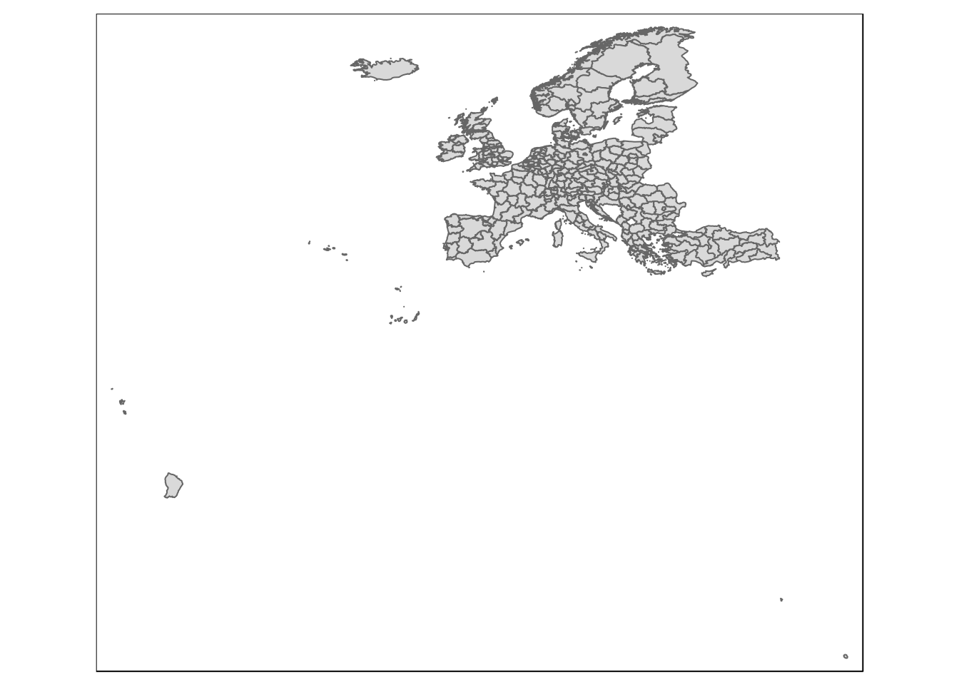
World
Various R packages containing spatial data for the entire world, e.g.:
- tmap: load using `data(“World”).
- rworldmap (regular resolution) and complementary package rworldxtra (high resolution)
library(tmap)
data("World")
world_tmap <- st_as_sf(World)
qtm(world_tmap)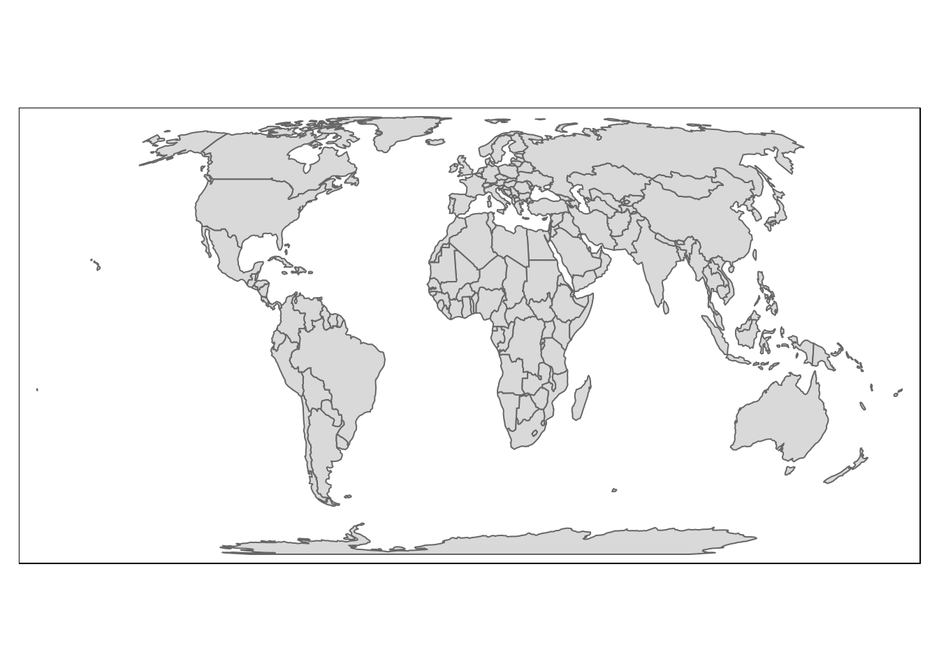
library(rworldmap)
#library(rworldxtra)

# load worldmap with resolution "coarse", "low", "less islands", "li", "high".
# for option "high" the additional package rworldxtra needs to be install, works the same.
world_worldmap <- getMap(resolution = "low")
world_worldmap <- st_as_sf(world_worldmap)
qtm(world_worldmap)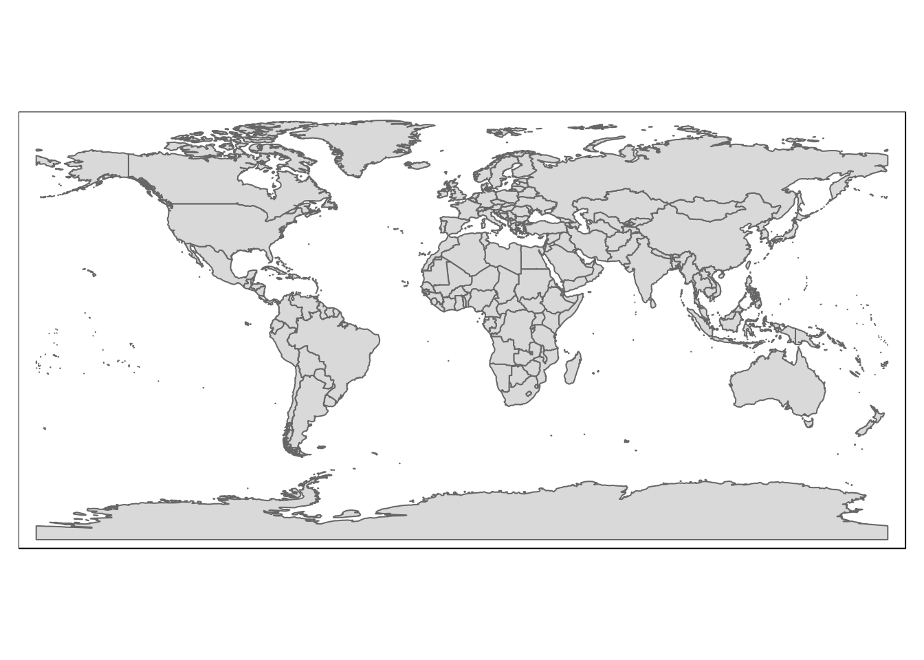
Get rid of too much map
Common situation, three options:
- Filter or select (un)wanted spatial data.
- Crop the map to the required area.
- Limit the visible map area.
Filter or select
Use a variable (originally in spatial dataset or added by you) to filter/select what you want from a larger map.
data("BE_ADMIN_PROVINCE")
prov <- st_as_sf(BE_ADMIN_PROVINCE)
qtm(prov)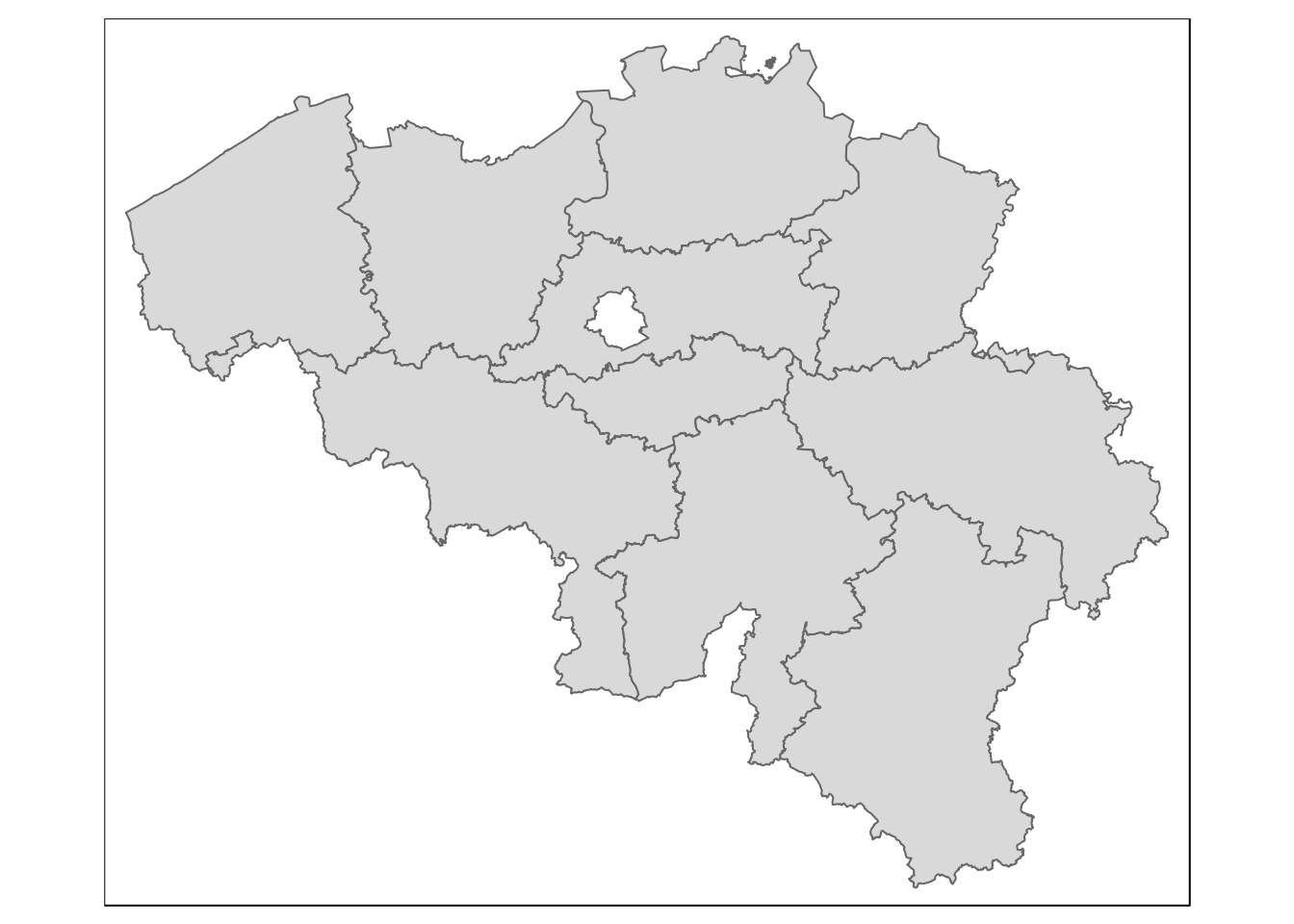
# filter out only the provinces in the region of Flanders, i.e.
# where the region description variable "TX_RGN_DESCR_NL" is equal to "Vlaams Gewest"
prov.fl <- prov %>%
  filter(TX_RGN_DESCR_NL == 'Vlaams Gewest')
qtm(prov.fl)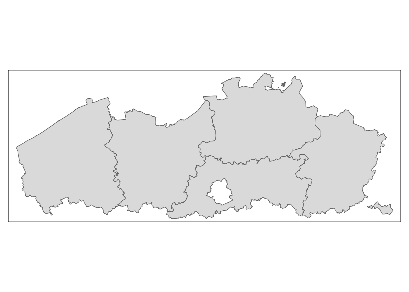
# filter out the South American countries from the world map
south_am <- world_worldmap %>%
  filter(GEO3 == 'South America')

qtm(south_am)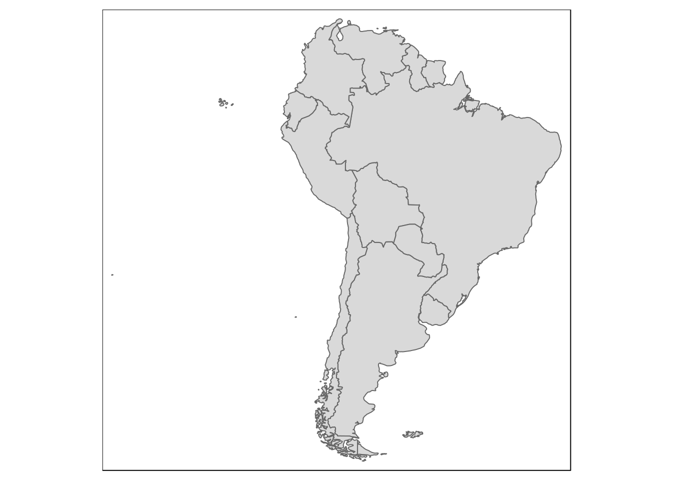
Limit visible area
Happens “at the end” when displaying the map, so depedent on what you use to display/plot. Example with tmap and ggplot:
qtm(eu_nuts2, bbox = 'France')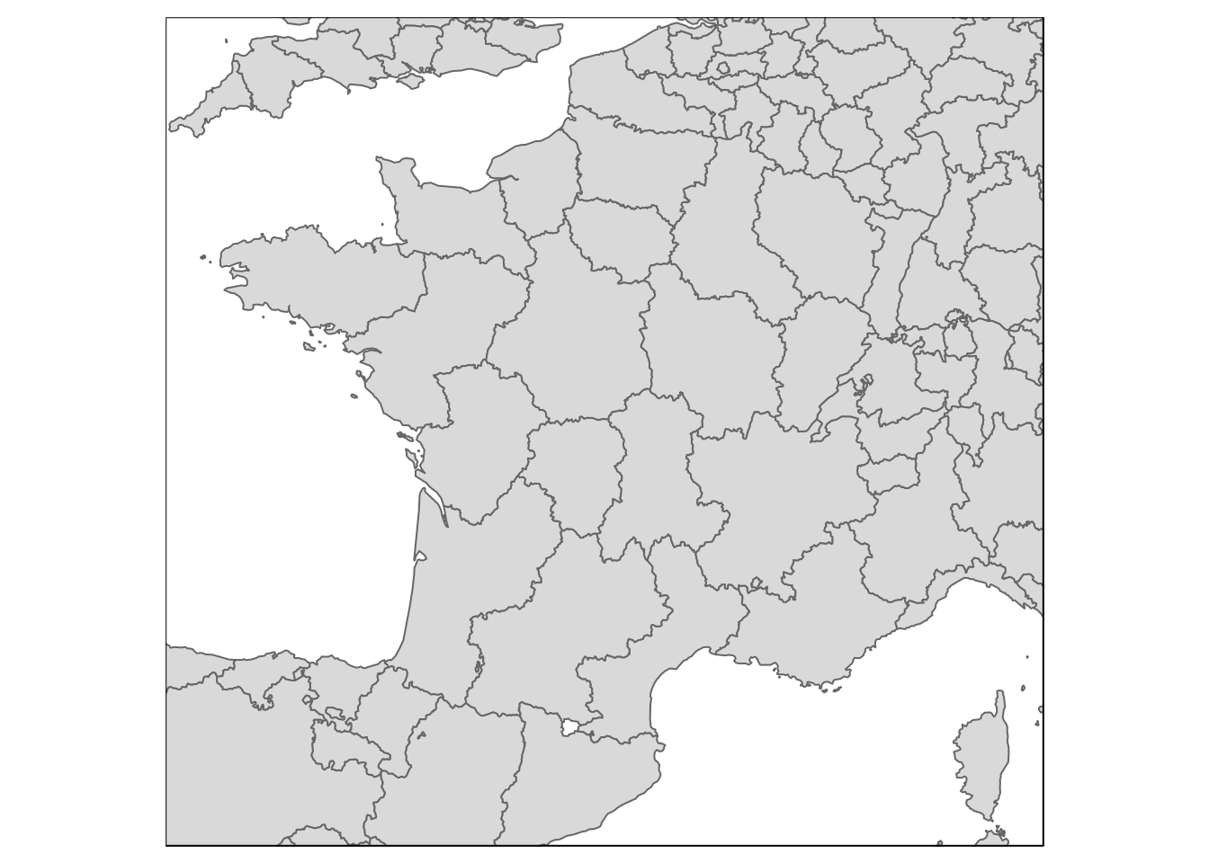
ggplot(eu_nuts0) +
  geom_sf() +
  coord_sf(
    # limit map to 'mainland' EU
    xlim = c(2500000, 6000000), ylim =c(1500000, 5300000),
    crs = 3035)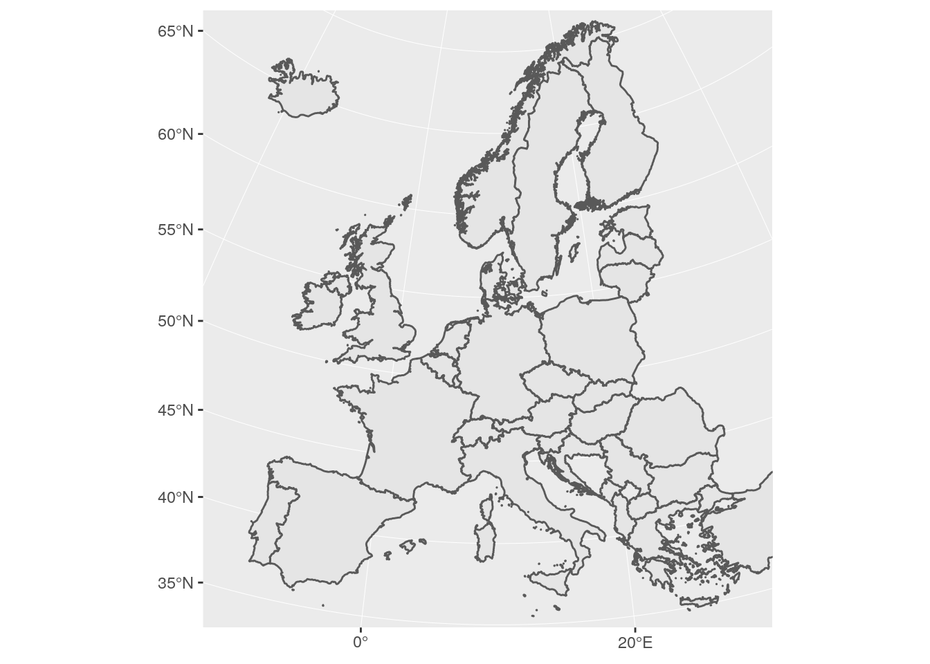
Crop spatial features
Use st_crop() from the sf package to crop a map to certain limits (remove rest)
eu <- st_crop(eu_nuts0, c(xmin=-10, xmax=45, ymin=36, ymax=71))
qtm(eu)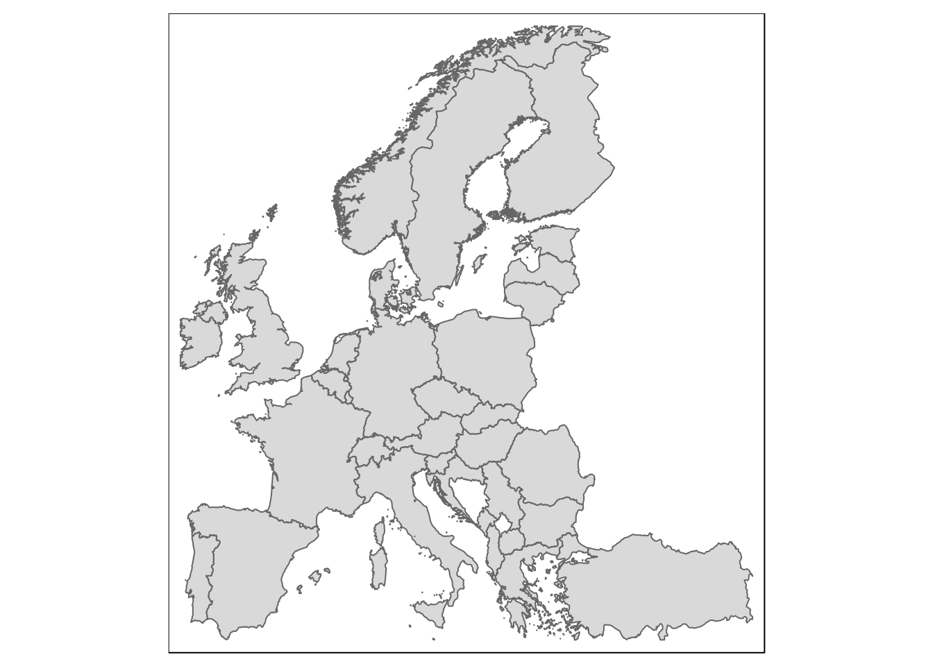
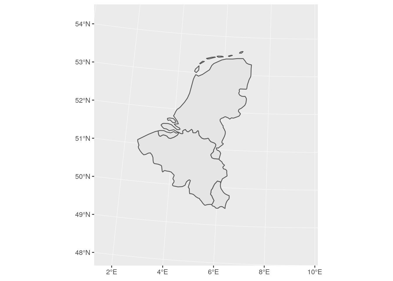
Combine filter, crop, limit
# Filter out the Benelux based on country-names
benelux <- world_worldmap %>%
  filter(NAME %in% c('Belgium', 'Netherlands', 'Luxembourg'))

# Plot Benelux and (exactly) limit map (decolonisation)
ggplot(benelux) +
  geom_sf() +
  coord_sf(xlim = c(3700000, 4300000),
           ylim =c(2800000, 3500000), crs = 3035)