Adding data
We have a spatial dataframe (see previous step 1), now we want to load and add our data-of-interest to visualise on the thematic map:
- Read in data-of-interst into R.
- Join data-of-interest with the spatial dataframe.
Crucial for linking spatial data and data-of-interest: have a variable/column in your that contains the appropriate spatial identifier. E.g. Census-identifer, NIS-code, NUTS-code, etc.
How to read in your data depends on the format, three recommended R-packages should cover mosts posibilities:
- readr: read/write plain text formats such as CSV, TXT, etc.
- readxl: read in Excel-files (.xlsx, .xls).
- haven: read/write datasets from SAS, SPSS, Stata.
library(here)
library(tidyr)
library(readxl)
library(dplyr)
library(sf)
library(tmap)
Read in data-of-interest: census 1851
# census 1851 datafile: 156.300 records x 11 variables
census_data <- read_xlsx(here('data/source/census1851_occupations_count.xlsx'))
# show records 1 to 10
census_data %>%
slice(1:10)## # A tibble: 10 x 11
## county_name district_name district_id sex occupation_label
## <chr> <chr> <dbl> <chr> <chr>
## 1 Bedfordshi… Ampthill 181 F agricultural la…
## 2 Bedfordshi… Ampthill 181 F annuitant
## 3 Bedfordshi… Ampthill 181 F baker
## 4 Bedfordshi… Ampthill 181 F blacksmith
## 5 Bedfordshi… Ampthill 181 F butchers wife
## 6 Bedfordshi… Ampthill 181 F charwoman
## 7 Bedfordshi… Ampthill 181 F cowkeeper, milk…
## 8 Bedfordshi… Ampthill 181 F dau, granddau, …
## 9 Bedfordshi… Ampthill 181 F domestic servan…
## 10 Bedfordshi… Ampthill 181 F domestic servan…
## # … with 6 more variables: occupation_count <dbl>, pst_a_code <dbl>,
## # pst_b_code <dbl>, pst_c_code <dbl>, pst_d_code <dbl>,
## # pst_a_label <chr>Explore data-of-interest
Exploring and manipulating data uses tidyverse “verbs”: filter, select, group_by, join, tally, mutate, etc.
Occupations & gender
# group records by gender, an tally up all persons
census_data %>%
  group_by(sex) %>%
  tally(occupation_count)
## # A tibble: 2 x 2
## sex n
## <chr> <dbl>
## 1 F 4775509
## 2 M 4399377# group by gender & and occupational category and tally
census_data %>%
group_by(sex, pst_a_label) %>%
tally(occupation_count) %>%
spread(sex, n)## # A tibble: 7 x 3
## pst_a_label F M
## <chr> <dbl> <dbl>
## 1 no_occupation 2698848 120789
## 2 primary 285660 1298589
## 3 secondary 762586 1730702
## 4 sector_unspecific 5001 249180
## 5 tertiary_dealers 18140 87801
## 6 tertiary_sellers 47306 119377
## 7 tertiary_services_professions 957968 792939# add a column with the percentage of women for each occupational group
census_data %>%
group_by(sex, pst_a_label) %>%
tally(occupation_count) %>%
spread(sex, n) %>%
mutate(pct_women = F / ( F + M) )## # A tibble: 7 x 4
## pst_a_label F M pct_women
## <chr> <dbl> <dbl> <dbl>
## 1 no_occupation 2698848 120789 0.957
## 2 primary 285660 1298589 0.180
## 3 secondary 762586 1730702 0.306
## 4 sector_unspecific 5001 249180 0.0197
## 5 tertiary_dealers 18140 87801 0.171
## 6 tertiary_sellers 47306 119377 0.284
## 7 tertiary_services_professions 957968 792939 0.547Which county has the most bakers in 1851?
census_data %>%
  filter(occupation_label == 'baker') %>% # select only records with occup 'baker'
  group_by(county_name) %>%
  tally(occupation_count) %>% # count bakers, grouped by county
  arrange(desc(n)) # sort descending on number of bakers
## # A tibble: 42 x 2
## county_name n
## <chr> <dbl>
## 1 London 10321
## 2 Lancashire 3503
## 3 Kent 1681
## 4 Devonshire 1552
## 5 Hampshire 1364
## 6 Somerset 1353
## 7 Gloucestershire 1338
## 8 Essex 1214
## 9 Warwickshire 1180
## 10 Yorkshire West Riding 1141
## # … with 32 more rowsPercentage secondary-sector workers per district
# make a new dataframe named districts_data with for
#  each district the counts per occupational category
districts_data <- census_data %>%
  group_by(district_id, district_name, pst_a_label) %>%
  tally(occupation_count) %>%
  spread(pst_a_label, n)

# calculate the percentage of people employed in secondary sector
districts_data <- districts_data %>%
  mutate(total = primary + secondary + tertiary_dealers + tertiary_sellers + tertiary_services_professions + sector_unspecific + no_occupation) %>%
  mutate(pct_secondary = secondary / total)

districts_data
## # A tibble: 576 x 11
## district_id district_name no_occupation primary secondary
## <dbl> <chr> <dbl> <dbl> <dbl>
## 1 1 Kensington 21466 2274 12367
## 2 2 Chelsea 10610 529 7884
## 3 3 St George Ha… 12506 256 8937
## 4 4 Westminster 12973 343 10535
## 5 5 St Martins-i… 4187 72 4198
## 6 6 St James Wes… 5795 123 7619
## 7 7 Marylebone 27911 1140 24945
## 8 8 Hampstead 1860 293 1009
## 9 9 Pancras 31016 943 28843
## 10 10 Islington 18193 933 13589
## # … with 566 more rows, and 6 more variables: sector_unspecific <dbl>,
## # tertiary_dealers <dbl>, tertiary_sellers <dbl>,
## # tertiary_services_professions <dbl>, total <dbl>, pct_secondary <dbl>Join spatial data (districts) and data-of interest (occupation-data)
Join spatial and non-spatial dataframes using general dataframe-join functions, cf. online cheatsheet for types of joins.
# Example syntax:
library(dplyr)
data <- left_join(spatial_data, data_of_interest, by = "identifier")
data <- left_join(spatial_data, data_of_interest, by = c("spatial_identifier" = "data_identifier"))
Example: join spatial data on districts, adding the counts and calculated percentages on occupations on district-level.
# load spatial data on districts
districts_spatial <- st_read(here('data/source/census_1851_districts/1851EngWalesRegistrationDistrict.shp')) %>%
  mutate(CEN1 = as.numeric(as.character(CEN1))) # make sure identifiers are the same type as in the district data
# add population data on district-level to the spatial data-set
districts <- left_join(districts_spatial, districts_data, by = c('CEN1' = 'district_id'))# single dataframe containing variables + spatial information (district boundaries) in geometry-column
districts## # A tibble: 1,198 x 17
## CEN1 R_DIST R_CTY R_DIVNO R_DIV R_CTRY district_name no_occupation
## <dbl> <fct> <fct> <fct> <fct> <fct> <chr> <dbl>
## 1 3 ST GE… LOND… I LOND… ENGLA… St George Ha… 12506
## 2 6 ST. J… LOND… I LOND… ENGLA… St James Wes… 5795
## 3 7 MARYL… LOND… I LOND… ENGLA… Marylebone 27911
## 4 8 HAMPS… LOND… I LOND… ENGLA… Hampstead 1860
## 5 10 ISLIN… LOND… I LOND… ENGLA… Islington 18193
## 6 11 HACKN… LOND… I LOND… ENGLA… Hackney 10897
## 7 12 ST GI… LOND… I LOND… ENGLA… St Giles 9990
## 8 14 HOLBO… LOND… I LOND… ENGLA… Holborn 8536
## 9 16 ST LU… LOND… I LOND… ENGLA… St Luke 9881
## 10 18 WEST … LOND… I LOND… ENGLA… West London 4836
## # … with 1,188 more rows, and 9 more variables: primary <dbl>,
## # secondary <dbl>, sector_unspecific <dbl>, tertiary_dealers <dbl>,
## # tertiary_sellers <dbl>, tertiary_services_professions <dbl>,
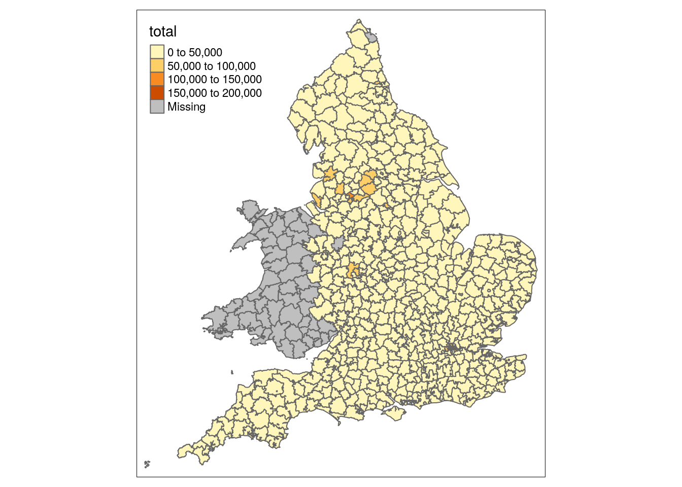
## # total <dbl>, pct_secondary <dbl>, geometry <POLYGON [m]>Test: display joined data on a map
# fill in the district boundaries with the total count of persons
qtm(districts, fill = 'total')